ECE 4750 Section 4 and 5: Lab 2 Head Start

Author: Cecilio C. Tamarit
Date: September 19, 2023
Based on previous material from Christopher Batten

Table of Contents

Replicating our setup locally
TinyRV2 Processor Walk-Through
Testing the ADD Instruction
Implementing and Testing the ADDI Instruction
Evaluating an Accumulate Function

This discussion section serves to introduce students to the basic processor modeling approach and testing strategy we will be using to implement a pipelined TinyRV2 processor in lab 2.

Replicating our setup locally

Before we start, many people have been asking how to replicate our setup for this class “at home.” As the complexity of the designs is increasing, we have deemed it particularly important to take a look at how that’s done. Running locally can be faster than using our shared ecelinux infrastructure.

Fortunately, our current setup is quite barebones, as this year we focused on streamlining. In fact, as we discussed in Section 2, our only actual dependency is Verilator itself (and, of course, its own prerequisites). The official Verilator documentation provides instructions on how it can be installed on all platforms, including a Windows version. However, to further simplify things, we recommend Windows users set up a virtual machine, or the WSL following this guide. That way, we can assume that everyone in this class has a Unix-like setup with mostly the same commands (e.g. an underlying Linux distro or macOS.)

For a performance boost, we first recommend installing Ccache, a compiler cache that will prevent redundant compilations of unchanged code, and mold (sold), a fast linker:

% sudo apt-get install ccache mold  # If on Linux with APT
% brew install ccache mold          # If on macOS with Homebrew

Verilator and all its dependencies could then be installed as follows:

% sudo apt-get install verilator    # If on Linux with APT
% brew install verilator            # If on macOS with Homebrew

Alternatively, Docker fans may resort to the official container.

However, to take advantage of the aforementioned performance improvements, we recommend that students install the latest version of Verilator (at the time this guide was published v5.0.16) by cloning it from the official repo and compiling it from source as follows:

% git clone https://github.com/verilator/verilator
% cd verilator
% autoconf
% ./configure
% make

For waveform visualization, you may resort to either:

GTKWave, which can be obtained here and will open FST, VCD, and other formats.
The Visual Studio Code + Plug-in approach we suggested in Section 3, which also works locally.

For the latter, note that the Makefile has been updated and there is no need to change anything. Just set the following environment variable before running anything:

% export VCD=1

To generate coverage reports, you have to make sure lcov is installed:

% sudo apt-get install lcov               # If on Linux with APT
% brew install lcov                       # If on macOS with Homebrew

Time to test that Makefile

The previous steps will allow you to run the commands in the Makefile we provide with each lab, which naturally depends on GNU Make, which is most likely already installed in your Linux distro / WSL / macOS, but just in case:

% sudo apt-get install build-essential    # If on Linux with APT
% brew install make                       # If on macOS with Homebrew

Of course, making use of our Makefiles requires setting the paths to where your local Verilator and compiler binaries are located. If the default ones don’t work, you can hardcode them by editing the Makefile or setting the environment variables (export VAR = value) so that:

VERILATOR_ROOT = /path/to/your/bin/verilator
VERILATOR_COVERAGE = /path/to/your/bin/verilator_coverage
CC = /path/to/your/bin/gcc
CXX = /path/to/your/bin/g++

With the variables set accordingly, go back to the directory containing all labs and as usual:

 % make setup

TinyRV2 Processor Walk-Through

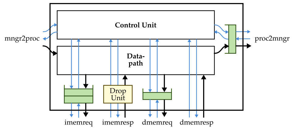
The following figure shows the high-level interface for our TinyRV2 processor. The processor has an independent instruction memory and data memory interface along with a mngr2proc and proc2mngr stream interface for testing purposes. All interfaces are implemented using the latency-insensitive val/rdy micro-protocol.

We provide students with a complete functional-level model of a processor that implements the above interface and can be used as a reference. You can find the FL model in lab2_proc/ProcFLMultiCycle.v.

Notice there are some extra ports to set the core id and for statistics, and that we are using SystemVerilog structs to encode the memory requests and responses. Here is the memory request struct format:

 76  74 73           66 65              34 33  32 31               0
+------+---------------+------------------+------+------------------+
| type | opaque        | addr             | len  | data             |
+------+---------------+------------------+------+------------------+

And here is the memory response struct format:

 46  44 43           36 35  34 33  32 31               0
+------+---------------+------+------+------------------+
| type | opaque        | test | len  | data             |
+------+---------------+------+------+------------------+

The full TinyRV2 instruction set includes the following instructions:

CSR: csrr, csrw
Reg-Reg: add, sub, mul, and, or, xor, slt, sltu, sra, srl, sll
Reg-Imm: addi, ori, andi, xori, slti, sltiu, srai, srli, slli, lui, auipc
Memory: lw, sw
Jump: jal, jalr
Branch: bne, beq, blt, bltu, bge, bgeu

In this discussion section, we provide you with a baseline processor implementation that implements ADD, LW, BNE, CSRR, and CSRW. The block diagram for how the control unit and datapath unit are composed is shown below.

The datapath for this simple processor is shown below.

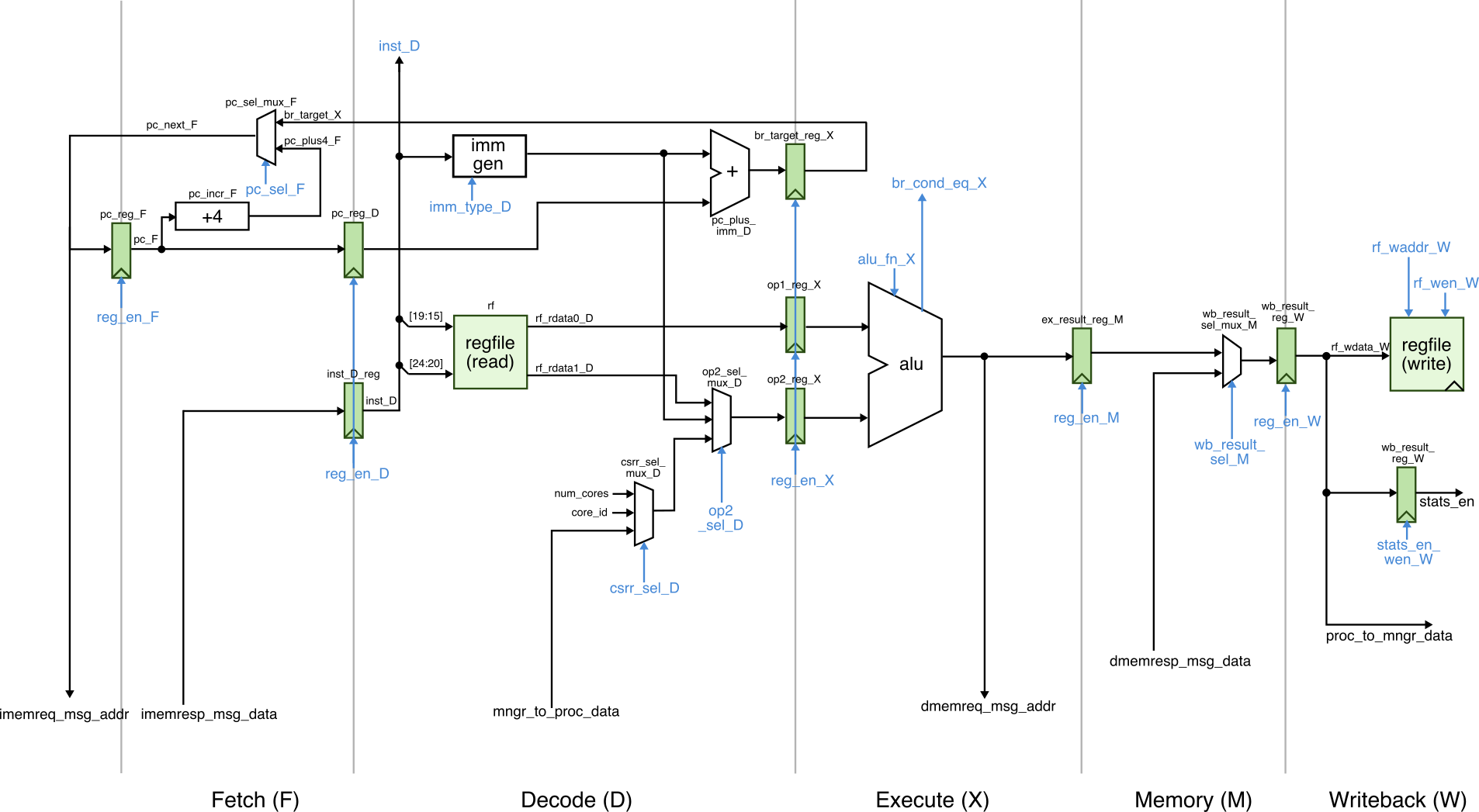
Your task in the first part of Lab 2 is to support the entire TinyRV2 ISA in this baseline processor.

Testing the ADD Instruction

Let’s take a look at a basic test for the ADD instruction. The primary way we will test our processors is by writing very small assembly test programs. Take a look at the test in lab2_proc/ams/add_alt.asm to see how to write such assembly test programs.

#---------------------------------------
# sample asm file for tutorial
#---------------------------------------

csrr x1, mngr2proc < 5
csrr x2, mngr2proc < 4
nop
nop
nop
nop
nop
nop
nop
nop
add x3, x1, x2
nop
nop
nop
nop
nop
nop
nop
nop
csrw proc2mngr, x3 > 9
nop
nop
nop
nop
nop
nop
nop
nop

There are two special control status registers (CSR) that we will use extensively in testing. If we read the mngr2proc CSR using a CSRR instruction, then this deques a message from the mngr2proc stream interface (the message comes from the stream source) and writes it to the given general purpose register. If we write the mngr2proc CSR using a CSRW instruction, then this enqueues a message onto the proc2mngr stream interface (the message goes to the stream sink). We can use the < symbol to specify in the assembly code what value we want the stream source to send to the processor for that instruction, and we can use the > symbol to specify in the assembly code what value we want the stream sink to check for that instruction.

You should always make sure your tests pass on the FL model before using them to test your baseline and alternative models. Let’s run the above test on our FL model.

% cd $TOPDIR/lab2_proc
% make add.hex
% make add.hex.sim DESIGN=ProcFLMultiCycle RUN_ARG=--trace

Use the --trace argument so you can see the linetrace. Verify that the instructions you think should be executing are indeed executing on the FL model. Now, let’s try the same test on the baseline processor:

% make add.hex.sim DESIGN=ProcBaseline RUN_ARG=--trace

The linetrace should look something like this:

 1r .        >          |                       |    |    |    |[ ]                         >                  [  ]| >
 2r .        >          |                       |    |    |    |[ ]                         >                  [  ]| >
.        >          |                       |    |    |    |[ ]rd:00:00000200:0:        >                  [  ]| >
#        >  00000200|                       |    |    |    |[ ]rd:00:00000204:0:        >rd:00:0:0:fc0020f3[ *]| >
00000005 >  00000204|csrr   x01, mngr2proc  |    |    |    |[ ]rd:00:00000208:0:        >rd:00:0:0:fc002173[ *]| >
00000004 >  00000208|csrr   x02, mngr2proc  |csrr|    |    |[ ]rd:00:0000020c:0:        >rd:00:0:0:00000013[ *]| >
.        >  0000020c|nop                    |csrr|csrr|    |[ ]rd:00:00000210:0:        >rd:00:0:0:00000013[ *]| >
.        >  00000210|nop                    |nop |csrr|csrr|[ ]rd:00:00000214:0:        >rd:00:0:0:00000013[ *]| >
.        >  00000214|nop                    |nop |nop |csrr|[ ]rd:00:00000218:0:        >rd:00:0:0:00000013[ *]| >
.        >  00000218|nop                    |nop |nop |nop |[ ]rd:00:0000021c:0:        >rd:00:0:0:00000013[ *]| >
.        >  0000021c|nop                    |nop |nop |nop |[ ]rd:00:00000220:0:        >rd:00:0:0:00000013[ *]| >
.        >  00000220|nop                    |nop |nop |nop |[ ]rd:00:00000224:0:        >rd:00:0:0:00000013[ *]| >
.        >  00000224|nop                    |nop |nop |nop |[ ]rd:00:00000228:0:        >rd:00:0:0:00000013[ *]| >
.        >  00000228|nop                    |nop |nop |nop |[ ]rd:00:0000022c:0:        >rd:00:0:0:002081b3[ *]| >
.        >  0000022c|add    x03, x01, x02   |nop |nop |nop |[ ]rd:00:00000230:0:        >rd:00:0:0:00000013[ *]| >
.        >  00000230|nop                    |add |nop |nop |[ ]rd:00:00000234:0:        >rd:00:0:0:00000013[ *]| >
.        >  00000234|nop                    |nop |add |nop |[ ]rd:00:00000238:0:        >rd:00:0:0:00000013[ *]| >
.        >  00000238|nop                    |nop |nop |add |[ ]rd:00:0000023c:0:        >rd:00:0:0:00000013[ *]| >
.        >  0000023c|nop                    |nop |nop |nop |[ ]rd:00:00000240:0:        >rd:00:0:0:00000013[ *]| >
.        >  00000240|nop                    |nop |nop |nop |[ ]rd:00:00000244:0:        >rd:00:0:0:00000013[ *]| >
.        >  00000244|nop                    |nop |nop |nop |[ ]rd:00:00000248:0:        >rd:00:0:0:00000013[ *]| >
.        >  00000248|nop                    |nop |nop |nop |[ ]rd:00:0000024c:0:        >rd:00:0:0:00000013[ *]| >
.        >  0000024c|nop                    |nop |nop |nop |[ ]rd:00:00000250:0:        >rd:00:0:0:7c019073[ *]| >
.        >  00000250|csrw   proc2mngr, x03  |nop |nop |nop |[ ]rd:00:00000254:0:        >rd:00:0:0:00000013[ *]| >
.        >  00000254|nop                    |csrw|nop |nop |[ ]rd:00:00000258:0:        >rd:00:0:0:00000013[ *]| >
.        >  00000258|nop                    |nop |csrw|nop |[ ]rd:00:0000025c:0:        >rd:00:0:0:00000013[ *]| >
.        >  0000025c|nop                    |nop |nop |csrw|[ ]rd:00:00000260:0:        >rd:00:0:0:00000013[ *]| > 00000009
.        >  00000260|nop                    |nop |nop |nop |[ ]rd:00:00000264:0:        >rd:00:0:0:00000013[ *]| >
.        >  00000264|nop                    |nop |nop |nop |[ ]rd:00:00000268:0:        >rd:00:0:0:00000013[ *]| >
.        >  00000268|nop                    |nop |nop |nop |[ ]rd:00:0000026c:0:        >rd:00:0:0:00000013[ *]| >
.        >  0000026c|nop                    |nop |nop |nop |[ ]rd:00:00000270:0:        >rd:00:0:0:00000013[ *]| >
.        >  00000270|nop                    |nop |nop |nop |[ ]rd:00:00000274:0:        >rd:00:0:0:fc0020f3[ *]| >

Implementing and Testing the ADDI Instruction

Now let’s add the ADDI instruction to our simple processor. It is critical to always take an incremental approach. Add a single instruction to your processor. Do lots of testing and only once you are confident you have covered all of the corner cases should you move on to adding another instruction.

Use the given handout to plan your implementation. Make sure you understand how the control signals are set for the ADD instruction. Draw any modifications you need to the datapath, add any control signals you need to the control signal table, and then fill out the row in the control signal table for the ADDI instruction. Here are the explanations of each control signal:

val : whether or not the instruction is valid; should be y for all instructions; basically a way to determine if this is a valid instruction or not for debugging purposes
br type : is either br_na if this is not a branch or br_bne if this is a BNE operation
imm type : immediate format corresponding to the TinyRV2 instruction set manual. imm_i is for I-type immediate format and imm_b is for B-type immediate format
rs1 en : set to n if this instruction does not use the rs1 field and set to y if this instruction does use the rs1 field; used for dependency checking
op2 muxsel : mux select control signal for the op2 mux; use bm_rf to choose the value from the register file, use bm_imm to choose the value from the immediate generation unit, use csr to choose the value from the CSR mux
rs2 en : set to n if this instruction does not use the rs2 field and set to y if this instruction does use the rs2 field; used for dependency checking
alu fn : ALU function control signal; use alu_add for the ALU to do an add; use alu_cp0 for the ALU to copy op0 to the output; use alu_cp1 for the ALU to copy op1 to the output
dmm type : the type of data memory operation; use nr if this is not a memory request; use ld if this is a load
wbmux sel : mux select control signal for writeback mux; use wm_a to choose the value from the ALU; use wm_m to choose the value from the data memory
rf wen : register file write enable; set to n if this instruction does not need to write the register file; set to y if this instruction does need to write the register file
csrr/csrw : whether this is a CSRR or CSRW instruction

Once you have the control signal table filled out on paper, go ahead and add a new row to the control signal table in lab2_proc/ProcBaseCtrl.v:

always_comb begin
  casez ( inst_D )
    //                            br      imm   rs1 op2    rs2 alu      dmm wbmux rf
    //                       val  type    type   en muxsel  en fn       typ sel   wen csrr csrw
    `TINYRV2_INST_NOP     :cs( y, br_na,  imm_x, n, bm_x,   n, alu_x,   nr, wm_a, n,  n,   n    );
    `TINYRV2_INST_ADD     :cs( y, br_na,  imm_x, y, bm_rf,  y, alu_add, nr, wm_a, y,  n,   n    );
    `TINYRV2_INST_LW      :cs( y, br_na,  imm_i, y, bm_imm, n, alu_add, ld, wm_m, y,  n,   n    );
    `TINYRV2_INST_BNE     :cs( y, br_bne, imm_b, y, bm_rf,  y, alu_x,   nr, wm_a, n,  n,   n    );
    `TINYRV2_INST_CSRR    :cs( y, br_na,  imm_i, n, bm_csr, n, alu_cp1, nr, wm_a, y,  y,   n    );
    `TINYRV2_INST_CSRW    :cs( y, br_na,  imm_i, y, bm_rf,  n, alu_cp0, nr, wm_a, n,  n,   y    );
  endcase
end

We can use the test asm file in lab2_proc/asm/addi.asm similar in spirit to the test cases we used to test the ADD instruction. Then run the test case on both ProcFL and ProcBase. Look at the final diff output to confirm your test case is doing what you expect on ProcBase.

% cd $TOPDIR/lab2_proc
% make addi.hex
% make addi.hex.diff DESIGN=ProcBase

Evaluating an Accumulate Function

Now let’s try to run the assembly for a simple C function on the simple processor and start to look at its performance. Write out the TinyRV2 assembly code that implements this C function:

int accumulate( int* a, int n )
{
  int sum = 0;
  for ( int i = 0; i < n; i++ ) {
    int b = a[i];
    sum   = sum + b;
  }
  return sum;
}

You should only use the instructions we have implemented in the simple processor (ADD, ADDI, LW, BNE). Once you have the assembly, save it to the lab2_proc/asm folder. Then try running the program on both ProcFL and ProcBase like this:

% cd $TOPDIR/build
% make accum.hex
% amke accum.hex.diff DESIGN=ProcBase

Take a look at the line trace to estimate the number of cycles per iteration.